
How tiny is TinyML? How fast is TinyML?
Do you want to get some REAL numbers on embedded machine learning on Arduino, STM32, ESP32, Seeedstudio boards (and more coming)?
This page will answer all your questions!
Background
If you're new to this blog, you need to know that (almost one year ago) I settled on a mission to bring machine learning to embedded microcontrollers of all sizes (even the Attiny85!).
To me, it is just insane to deploy heavyweight Neural Networks to such small devices, if you don't need their expressiveness (mainly image and audio analysis). The vast majority of embedded ML tasks is, in fact, related to sensors' readings, which can easily be solved with "traditional" ML algorithms.
Today's industry seems to be more leaned toward Neural Networks, though, so I thought it would be beneficial for you readers to get an actual grasp on the potential of traditional Machine learning algorithms in the embedded context.
On this blog you can find posts about:
- Decision Tree, Random Forest and XGBoost
- Gaussian Naive Bayes
- SEFR - a binary classifier
- PCA for dimensionality reduction
- Relevant Vector Machines
- SVM for gesture detection
- One Class SVM for anomaly detection
All these algorithms go a long way in both accuracy and resource comsumption, so (in my opinion) they should be your first choice when developing a new project.
To support my claimings I made a huge effort to collect real world data, and now I want to share this data with you.
Before you ask:
"Are Neural Networks models benchmarked here?". No.
"Will Neural Networks model be benchmarked in the future?". Yes, as soon as I'm comfortable with them: I want to create a fair comparison between NN and traditional algorithms.
So now let's move to the contents.
The boards
I run the benchmarks on the boards I have at hand: they were all purchased by me, except for the Arduino Nano BLE Sense (given to me by the Arduino team).
- Espressif ESP32
- Espressif ESP8266 NodeMCU v1.0
- STM32 Nucleo L432KC (Cortex M4)
- Seeedstudio XIAO (SAMD21 Cortex M0)
- Arduino Nano 33 BLE Sense (Cortex M4F)
The datasets
I picked a small selection of toy and real world datasets to benchmark the classifiers against (the real world ones were picked from a TinyML Talks presentation when easily available, plus some more from the UCI database almost at random).
Here's the list of the benchmarked datasets, with the shape of the dataset (in the format number of samples x number of features x number of classes).
- Iris
(150 x 4 x 3): from the sklearn package - Wine
(178 x 13 x 3): from the sklearn package - Digits
(1797 x 64 x 10): from the sklearn package - Human Activity
(10299 x 561 x 6) - Sport Activity
(4800 x 180 x 10) - Gas Sensor Array Drift
(1000 x 128 x 6) - EMG
(1648 x 63 x 5 ) - Gesture Phase Segmentaion
(1000 x 19 x 5) - Statlog (Vehicle Silhouettes)
(846 x 18 x 4) - Mammographic Mass
(830 x 4 x 2) - Sensorless Drive Diagnosis
(1000 x 48 x 11)
The datasets are chosen to be representative of different domains and the list will grow in the next weeks.
Some datasets are used as-is, others were pre-processed with very light feature extraction. In detail:
Human Activityfeatures were extracted with a rolling window, and for each window min/max/avg/std/skew/kurtosis were calculatedSport Activitygot the same pre-processing, and the number of actvities was reduced from 19 to 10EMGfeatures were extracted with a rolling window, and for each window the Root Mean Square value was calculated
The reported benchmarks only consider the inference process: any feature extraction is not included! Nevertheless, only features with linear time complexity were used, so any MCU will have no problem in computing them.
The classifiers
The following classifiers are benchmarked:
- Decision Tree
- Random Forest
- XGBoost
- Logistic Regression
- Gaussian Naive Bayes
Why these classifiers?
Because they're all supported by the micromlgen package, so they can easily be ported to plain C.
* XGBoost porting failed on some datasets, so you will see holes in the data. I will correct this in the next weeks
micromlgen actually supports Support Vector Machines, too: it is not included because on real world datasets the number of support vector is so high (hundreds or even thousands) that no single board could handle that.
If you want to stay up to date with the new numbers, subscribe to the newsletter: I promise you won't receive more than 1 mail per month.
The Results
This section reports (a selection of) the charts generated from the benchmark results to give you a quick glance of the capabilities of the aforementioned boards and algorithms in terms of performance and accuracy.
If you like an interactive view of the data, there's a Colab Notebook that reproduces the charts reported here, where you can interact with the data as you like.
At the very end of the article, you can also find a link to the raw CSV file I generated (as you can see, it required A LOT of work to create).
Accuracy
The overall accuracy of each classifier on each dataset (this plot is not bounded to any particular board, it is computed "offline").
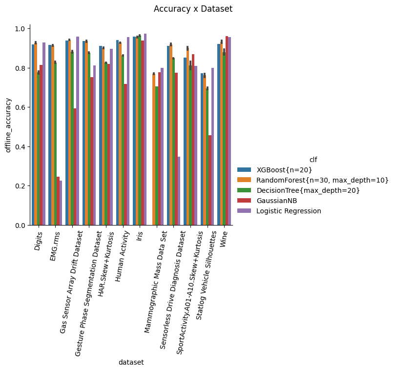
Comment: many classifiers (Random Forest, XGBoost, Logistic Regression) can easily achieve up to 95+ % accuracy on some datasets with minimal pre-processing, while still scoring 85+ % on more difficult datasets.
Flash percent
These charts plot, for each dataset, how much flash (in percent on the total available) it takes for the classifier to compile (visit the Colab Notebook to see all the charts).
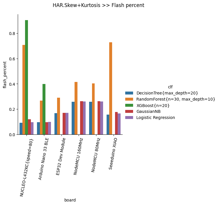
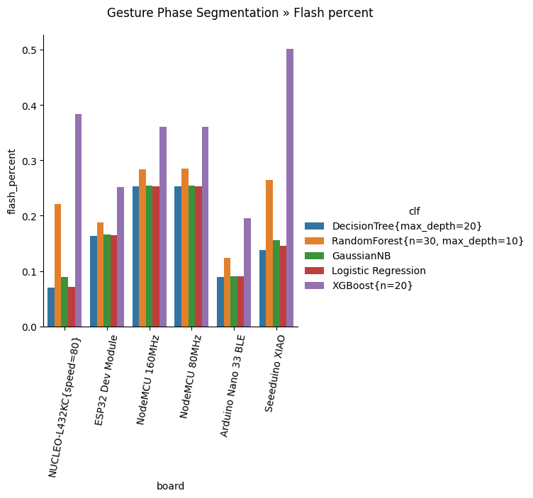
Comment: DecisionTree, GaussianNB and Logistic Regression require the least amount of flash. XGBoost is very "flash-intensive"; RandomForest sits in the middle.
How tiny can TinyML be?
As low as 6% of flash size for a fully functional DecisionTree with 85+% accuracy.
Inference time
These charts plot, for each dataset, how long it takes for the classifier to run (only the classification, no feature extraction!).
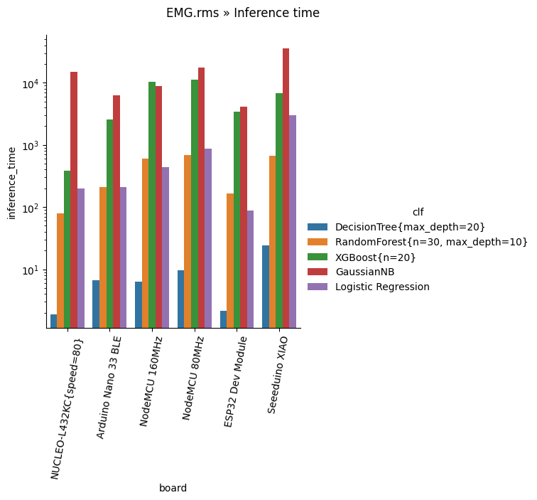
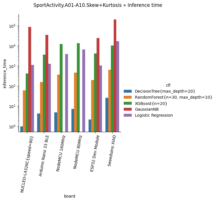
Comment: DecisionTree is the clear winner here, with minimal inference time (from 0.4 to 30 microseconds), followed by Random Forest. Logistic Regression, XGBoost and GaussianNB are the slowest.
How fast can TinyML be?
As fast as sub-millisecond inference time for a fully functional DecisionTree with 85+% accuracy.
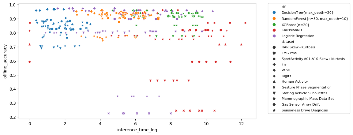
Inference time vs Accuracy
This plot correlates the inference time vs the classification accuracy. The more upper-left a point is, the better (fast inference time, high accuracy).
Click here to open the image at full size
Comment: as already stated, you will see a lot of blue markers (Decision Tree) in the top left, since it is very fast and quite accurate. Moving to the right you can see purple (Logistic Regression) and orange (Random Forest). GaussianNB (red) exhibits quite low accuracy instead.
Inference time vs Flash percent
This plot correlates the inference time vs the the (relative) flash requirement. The more lower-left a point is, the better (fast inference time, low flash requirements).
Click here to open the image at full size
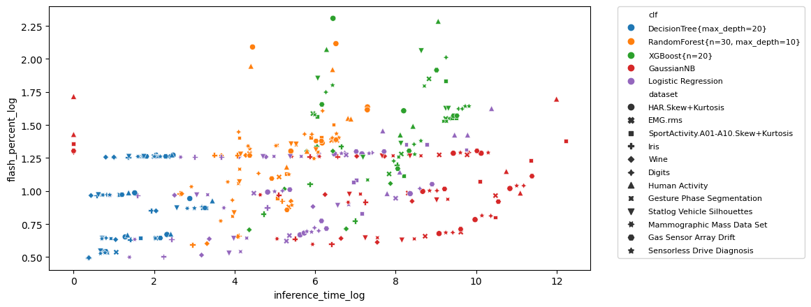
Comment: Again, we see blue (Decision Tree) is both fast and small, followed by Logistic Regression and Random Forest. Now it is clear that XGBoost (green), while not being the slowest, is the more demanding in terms of flash.
Conclusions
I hope this post helped you broaden your view on TinyML, on how tiny it can be, how fast it can be (sub-millisecond inference!), how wide it is.
Please don't hesitate to comment with your opinion on the subject, suggestions of new boards or datasets I should benchmark, or any other idea you have in mind that can contribute to the purpose of this page.
And don't forget to stay tuned for the updates: I already have 2 more boards I will benchmark in the next days!
As promised, here's the link to the raw benchmarks in CSV format.
You can run your own analysis and visualization on it: if you use it in your own work, please add a link to this post.
In future posts I will share how I collected all those numbers, so subscribe to the newsletter to stay up to date!